
or, how my love for video games and AI/ML brought me to an intersection of them with reinforcement learning.
The information in this post is not intended to be a thorough mathematical primer on the topic. Rather, it is simply to showcase and explain a cool concept I’ve learned and implemented myself, and to explain it to a layman. I will be discussing some math here and there, but I recommend the Reinforcement Learning book by Sutton and Barto if you’re really looking to get your hands dirty.
Introduction#
A common prank my friends and I like to conduct is to bring people to a game of Mao. Essentially, the uninitiated are not allowed to know the rules of this card game. They must figure it out by watching other people, and they usually end up suffering in-game penalties frequently as a result.
How would you approach this game (or, for the initiated, how did you first approach this game)? I bet that when starting the game, you would do a random move and see where that gets you. You would observe when you get penalized for something, and try to associate that pattern so that you try not to let it happen again. You might guess wrong, and then try a slightly tweaked version of your move to see if it happens again. Similarly with video games, I do the same thing: see what works, see what doesn’t, and try to keep doing what works and what doesn’t work. Lord knows how many times that I, someone who’s never played DnD before, tried to adjust my Baldur’s Gate 3 classes, actions, and story paths to get the most satisfying one across multiple playthroughs.
Definition#
This, my friends, is the essence of reinforcement learning: how an agent conducts actions in an environment to maximize its overall reward. We’ll get into what these terms mean in a second.
A very common image that gets utilized when describing RL is as follows: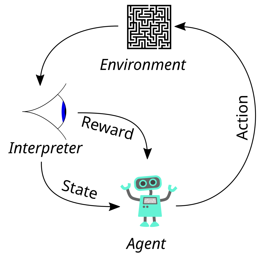
If you recognize what shape this takes, you are correct in assuming that this is a Markov decision process. If you don’t, no worries.
Let’s break this picture down piece by piece. You have an agent (a model, a piece of code, etc.) that takes an action and interacts with its environment. Then, the agent is given two pieces of input from the interpreter (a fancy way of saying something that translates the outcomes of the action to the environment). The state, which you can think of a snapshot of the environment after the action, and the reward, which is an incentive to the model. For an RL algo trading stocks, the reward in simple terms could be its profits. For checkers, the number of pieces captured. In the case of Mao, the reward would be… well. Wouldn’t you like to know? We then loop this process, and keep learning.
Note: the results of the prior action does not impact the probability of choosing the current action. Just a bit of a disclaimer before we move forward.
By this point, I’m sure you’ve been understanding everything I’ve said; however, one question probably still remains. “How?” And that, my friends, is what the next section is for. We’ll discuss an algorithm that I implemented!
Q-Learning#
Lots of people I know feel like this whenever they encounter/encountered a math test:
The Algo#
Don’t worry! I will do my best to walk you through the math. (If you weren’t worrying at all, then that’s good) Here’s the equation for the algorithm we’re going to cover today, Q-learning:
$$Q(S_t, A_t) \leftarrow Q(S_t, A_t) + \alpha \left[ R_{t+1} + \gamma \max_a Q(S_{t+1}, a) - Q(S_t, A_t) \right]$$
You see the \(Q(S_t, A_t)\). The \(Q\) is a function that we call a Q table. This is defined as follows: $$Q(s, a) = \mathbb{E}[R_t \mid S_t = s, A_t = a]$$
where the inputs to the Q table are the state s and action a that the agent takes. The \(\mathbb{E}\) refers to the expected value, \(R_t\) refers to the total reward up to the timestep (basically, what point of time we are in) t, and \(S_t\) and \(A_t\) are the state and action at timestep t. What does this mean? Basically: the Q table is keeping track of the cumulative reward up to time t for every (state, action) pair. Think about it: it’s basically what you do in a game you don’t know, right? You try something (action) in a certain situation (state) and see what that does for you (reward/no reward/sometimes negative reward). The Q table is a convenient way of keeping track of this.
Now, you’ll probably have seen already that the original Q learning algorithm updates itself. That’s cool, right? That’s how this model learns. Now that you have an understanding of the Q table, let’s go into the rest of the equation.
As we already covered, \(Q(S_t, A_t)\) is basically the current estimate of the reward for the (state, action) pair at time t. What about the \(\left[R_{t+1} + \gamma \max_a Q(S_{t+1}, a) - Q(S_t, A_t) \right]\)? \(R_{t+1}\) is essentially the reward after the action was done at timestep t, and the \(\gamma\) is the discount factor (we will get into this in a bit). The \(\max_a Q(S_{t+1}, a)\) is giving us the maximum possible reward for the next state at timestep t+1 after the corresponding action was done at time t; I know that was a mouthful, but basically, we’re figuring out which action a at timestep t gives us the best reward for the next state, and we’re rolling with that. The sum of these two terms is the target value. Our reward at this spot, plus the discounted future reward given that we take that action.
If you’ve taken a finance class before, you’ve probably learned about the time value of money. Essentially, $100 today is worth more than $100 next year. Why? The simple answer is opportunity cost. However, if you aren’t satisfied with that answer, or desire a more technical proof/explanation, feel free to look for one. We apply this opportunity cost with \(\gamma\), our discount factor. We discount future rewards, since the present rewards are worth much more, hence the multiplication. As you can guess from the explanation, the discount factor is usually between 0 and 1, though closer to 1. We don’t want to discount it TOO much.
Subtracting the original \(Q(S_t, A_t)\) gives us something called the *temporal difference (TD) error. Basically, we’re seeing how far away our current Q value in the table is to the target value (which is the sum of the reward and the discounted max possible future reward that we discussed earlier).
We then multiply this whole thing by the \(\alpha\), the learning rate. We don’t want to immediately swap out our Q table values to this one! We want to gradually make our way there, because we have no idea if what we’ve learned is exactly true or not. Similar to our Mao example: you don’t know if the reason you didn’t get penalized is completely due to you guessing the right rule. You might have gotten lucky! So you remember it, and keep an eye out for it next time, adjusting your expectations accordingly. You’ve by now deduced that the learning rate is a value between 0 and 1, but closer to 0, since you don’t want to update your values too quickly.
Now, for the final part. You adjust the \(Q(S_t, A_t)\) by adding what was in there previously with the learning rate times the TD error! This gives our Q value a little nudge in the right direction.
Implementation Explanation#
But “wait!”, you might say. How do we even start? Looking at the diagram earlier, it looked like a never ending loop. When do we start, and when do we stop? How do we make Q values in the first place? Let’s get into that too.
Let’s answer the easier questions first.
- When we start this, we initialize our current state to 0s (or nulls, depdending on how you would like to implement this), and we initialize our Q table to have all 0s as well.
- Starting and stopping involves two things: number of episodes, and the number of time steps per episode. What’s happening here is that each episode is the number of times we let the agent explore the environment (or, more simply, play the game) and the number of time steps is essentially the total amount of time we give the agent per episode.
Sure, that’s all cool. But what happens if the Q table contains all zeroes? How do we even start populating it with values? That’s a good question. We’re going to get into something called an epsilon (\(\epsilon\)) greedy strategy.
\(\epsilon\) Greedy Strategy#
Let’s go back to the initial discussion of the game of Mao. When you start playing the game, you don’t know anything except what your options are, which are to essentially put a card from your hand down. That’s all you know. From there, you randomly experiment and try to see what works and what doesn’t work. After you’ve gotten a hang of the game, however, you don’t want to keep doing random stuff: you want to go ahead and try to use what you know to win. This is known as exploration/exploitation.
When our agent first starts interacting with the environment, let’s give it some freedom to just randomly explore and try things and see what that gives it. However, as the agent gets a hang of things as it plays through a good number of episodes, we want it to exploit what it has learned in its Q table for the max possible reward.
This can be done through any sort of setup. It’s really up to you regarding how you wish to set this up, as long as it achieves the goal of decreasing your \(\epsilon\) (exploration/exploitation coefficient) over the episodes so the agent can first explore, then exploit. Here is my implementation: $$\epsilon \leftarrow \epsilon_{\text{min}} + (\epsilon_{\text{max}} - \epsilon_{\text{min}}) \cdot e^{(-d\cdot p)}$$
Where p is the episode number, \(\epsilon\) and \(\epsilon_{\text{max}}\) start off initialized as 1, and \(\epsilon_{\text{min}}\) and d (\(\epsilon\) decay: the rate at which the \(\epsilon\) value decreases) are usually initialized to values that are between 0 and 1, but usually much closer to 0. You can probably intuit that as the episodes go on, the \(\epsilon\) value decreases. But how do we use this? Simple, really.
Every time step, we pick a random number between 0 and 1. If this number is greater than \(\epsilon\), we just use whatever is in our Q table and make the decision from what we’ve seen. However, if it’s less than or equal to our \(\epsilon\) value, then we just randomly pick an action and roll with it, and see what that gives us.
Once again, you’ll be able to intuit that the first case probably happens later on in the episodes, while the second case happens towards the beginning of the episodes. We’re done with the theory!
Mess w/My Code!#
You might not have a perfect grasp on the algorithm yet, especially if you haven’t recently been studying or doing math. That’s okay. Seeing it in code form will help you out there.
We’re going to be using Gymnasium to help us set up. We’re going to be using their Cart-Pole game.
What’s happening here, and why did I choose this environment to do Q learning in?
Cart-pole is a famous intro for those who are dipping their feet into due to its simplicity. Basically, you are given a cart with a pendulum on top of it. The cart rolls on a frictionless surface. The action space (what all can the agent possibly do here?) is simple: push the cart left, and push the cart right. The objective is simple: keep the pendulum up for as long as possible. It’s considered a “fail” if the pendulum falls below a certain angle.
Here’s my GitHub repo for my Q learning implementation of cart-pole. Read through the file, see if you can understand it and try to rewrite it yourself. I’ve included some comments explaining stuff, as well as links to the documentation if you want to understand it more. Don’t hesitate to leave a comment if there’s anything you’re confused about.
Installation/Prereqs#
Last blog post was Hugo. This one is Python. Ensure that you have Python and pip installed, and then run the following commands. Note, this is assuming that you’re not using conda.
pip install gymnasium
pip install numpy
pip install matplotlib
git clone https://github.com/vajralakushal/cart-pole.git
Now, cd into the directory of the cart-pole and run:
python cart-pole-q.py
I’ve given you the option to select some paramters. Once you do, the model takes some time to train, and then a pyplot window should show up, plotting the average reward of the agent across every thousand episodes. Can you come up with a set of parameters where the cart-pole survives the longest (i.e. where the graph has the highest points).
Sources#
Huge shoutout to the videos in this playlist. Heavily inspired me to write my own intro to this topic. Everything else is linked accordingly.
Thanks!#
Thanks for reading! Feel free to leave any comments if you have any!